3. Autoencoders and anomaly detection
This section explores the potential usage of autoencoders in the context of credit card fraud detection.
3.1. Definition and usage
An autoencoder is a special type of deep learning architecture used to learn representations of data based solely on descriptive features. The representation, which is a transformation of the raw data, is learned with the objective to reconstruct the original data the most accurately. This representation learning strategy can be used for dimensionality reduction, denoising, or even generative applications.
An autoencoder can be divided into two parts:
The encoder part that maps the input into the representation, also referred to as the “code” or the “bottleneck”.
The decoder that maps the code to a reconstruction of the input.
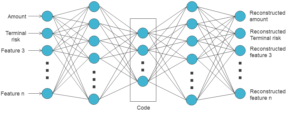
The encoder and decoder can have complex architectures like recurrent neural networks when dealing with sequential data or convolutional neural networks when dealing with images. But in their simplest form, they are multi-layer feed-forward neural networks. The dimension of the code, which is also the input of the decoder, can be fixed arbitrarily. This dimension is generally chosen to be lower than the original input dimension to reduce the dimensionality and to learn underlying meta variables. The dimension of the output of the decoder is the same as the input of the encoder because its purpose is to reconstruct the input.
The architecture is generally trained end-to-end by optimizing the input reconstruction, i.e. by minimizing a loss that measures a difference between the model’s output and the input. It can be trained with any unlabeled data. Note that when the autoencoder is “deep”, i.e. there are intermediate layers \(h_2\) and \(h_2'\) respectively between the input \(x\) and the bottleneck \(h\) and between the bottleneck and the output \(y\) (like in the figure above), one can train the layers successively instead of simultaneously. More precisely, one can first consider a submodel with only \(x\), \(h_2\) and \(y\) and train it to reconstruct the input from the intermediate code \(h_2\). Then, consider a second submodel with only \(h_2\), \(h\) and \(h_2'\) and train it to reconstruct the intermediate code from the code \(h\). Finally, fine-tune the whole model with \(x\), \(h_2\), \(h\), \(h_2'\) and \(y\) to reconstruct the input.
Autoencoders can be used as techniques for unsupervised or semi-supervised anomaly detection, which led them to be used multiple times for credit card fraud detection [AC15, ZP17].
3.1.1. Anomaly detection
Although not detailed before, fraud detection can be performed with both supervised and unsupervised techniques [CLBC+19, VAK+16], as it is a special instance of a broader problem referred to as anomaly detection or outlier detection. The latter generally includes techniques to identify items that are rare or differ significantly from the “normal” behavior, observable in the majority of the data.
And one can easily see how a credit card fraud can be defined as an anomaly in transactions. These anomalies can be rare events or unexpected bursts in the activity of a single cardholder behavior, or specific patterns, not necessarily rare, in the global consumers’ behavior. Rare events or outliers can be detected with unsupervised techniques that learn the normality and which are able to estimate discrepancy to this normality. But detection of other types of anomaly can require supervised techniques with proper training.
Therefore, one can think of three types of anomaly detection techniques:
Supervised techniques that were widely explored in previous sections and chapters. These techniques require annotations on data that consist of two classes, “normal” (or “genuine”) and “abnormal” (or “fraud”), and they learn to discriminate between those classes.
Unsupervised techniques that aim at detecting anomalies by modeling the majority behavior and considering it as “normal”. Then they detect the “abnormal” or fraudulent behavior by searching for examples that do not fit well to the normal behavior.
Semi-supervised techniques that are in between the two above cases and that can learn from both unlabeled and labeled data to detect fraudulent transactions.
An autoencoder can be used to model the normal behavior of data and detect outliers using the reconstruction error as an indicator. In particular, one way to do so is to train it to globally reconstruct transactions in a dataset. The normal trend that is observed in the majority of transactions will be better approximated than rare events. Therefore, the reconstruction error of “normal” data will be lower than the reconstruction error of outliers.
An autoencoder can therefore be considered as an unsupervised technique for fraud detection. In this section, we will implement and test it for both semi-supervised and unsupervised fraud detection.
3.1.2. Representation learning
Other than unsupervised anomaly detection, an autoencoder can simply be used as a general representation learning method for credit card transaction data. In a more complex manner than PCA, an autoencoder will learn a transformation from the original feature space to a representation space with new variables that encodes all the useful information to reconstruct the original data.
If the dimension of the code is chosen to be 2 or 3, one can visualize the transaction in the novel 2D/3D space. Otherwise, the code can also be used for other purposes, like:
Clustering: Clustering can be performed on the code instead of the original features. Groups learned from the clustering can be useful to characterize the types of behaviors of consumers or fraudsters.
Additional or replacement variables: The code can be used as replacement variables, or additional variables, to train any supervised learning model for credit card fraud detection.
3.1.3. Content of the section
The following puts into practice the use of autoencoders for credit card fraud detection. It starts by defining the data structures for unlabeled transactions. It then implements and evaluates an autoencoder for unsupervised fraud detection. The autoencoder is then used to compute transaction representation for visualization and clustering. Finally, we explore a semi-supervised strategy for fraud detection.
Let us dive into it by making all necessary imports.
# Initialization: Load shared functions and simulated data

# Load shared functions
!curl -O https://raw.githubusercontent.com/Fraud-Detection-Handbook/fraud-detection-handbook/main/Chapter_References/shared_functions.py
%run shared_functions.py

# Get simulated data from Github repository
if not os.path.exists("simulated-data-transformed"):
    !git clone https://github.com/Fraud-Detection-Handbook/simulated-data-transformed
This section reuses some “deep learning” specific material that was implemented in the previous section. It includes the evaluation function, the preparation of generators, the early-stopping strategy, the training loop, and so on. This material has been added to the shared functions.
3.2. Data loading
The same experimental setup as the previous section is used for our exploration, i.e. a fixed training and validation period, and the same features from the transformed simulated data (simulated-data-transformed/data/).
DIR_INPUT='simulated-data-transformed/data/'

BEGIN_DATE = "2018-06-11"
END_DATE = "2018-09-14"

print("Load  files")
%time transactions_df=read_from_files(DIR_INPUT, BEGIN_DATE, END_DATE)
print("{0} transactions loaded, containing {1} fraudulent transactions".format(len(transactions_df),transactions_df.TX_FRAUD.sum()))

output_feature="TX_FRAUD"

input_features=['TX_AMOUNT','TX_DURING_WEEKEND', 'TX_DURING_NIGHT', 'CUSTOMER_ID_NB_TX_1DAY_WINDOW',
       'CUSTOMER_ID_AVG_AMOUNT_1DAY_WINDOW', 'CUSTOMER_ID_NB_TX_7DAY_WINDOW',
       'CUSTOMER_ID_AVG_AMOUNT_7DAY_WINDOW', 'CUSTOMER_ID_NB_TX_30DAY_WINDOW',
       'CUSTOMER_ID_AVG_AMOUNT_30DAY_WINDOW', 'TERMINAL_ID_NB_TX_1DAY_WINDOW',
       'TERMINAL_ID_RISK_1DAY_WINDOW', 'TERMINAL_ID_NB_TX_7DAY_WINDOW',
       'TERMINAL_ID_RISK_7DAY_WINDOW', 'TERMINAL_ID_NB_TX_30DAY_WINDOW',
       'TERMINAL_ID_RISK_30DAY_WINDOW']
Load  files
CPU times: user 387 ms, sys: 282 ms, total: 669 ms
Wall time: 760 ms
919767 transactions loaded, containing 8195 fraudulent transactions
# Set the starting day for the training period, and the deltas
start_date_training = datetime.datetime.strptime("2018-07-25", "%Y-%m-%d")
delta_train=7
delta_delay=7
delta_test=7


delta_valid = delta_test

start_date_training_with_valid = start_date_training+datetime.timedelta(days=-(delta_delay+delta_valid))

(train_df, valid_df)=get_train_test_set(transactions_df,start_date_training_with_valid,
                                       delta_train=delta_train,delta_delay=delta_delay,delta_test=delta_test)

# By default, scales input data
(train_df, valid_df)=scaleData(train_df, valid_df,input_features)
3.3. Autoencoder implementation
For the sake of consistency, the implementation of the autoencoders will be done with the PyTorch library. As usual, a seed will be used as follows to ensure reproducibility:
SEED = 42

if torch.cuda.is_available():
    DEVICE = "cuda"
else:
    DEVICE = "cpu"
print("Selected device is",DEVICE)

seed_everything(SEED)
Selected device is cuda
Let us also convert our features and labels into torch tensors.
x_train = torch.FloatTensor(train_df[input_features].values)
x_valid = torch.FloatTensor(valid_df[input_features].values)
y_train = torch.FloatTensor(train_df[output_feature].values)
y_valid = torch.FloatTensor(valid_df[output_feature].values)
The autoencoder has the same input as the baseline feed-forward neural network but a different output. Instead of the fraud/genuine label, its target will be the same as the input. Therefore, the experiments here will not rely on the FraudDataset defined before but on a new Dataset: FraudDatasetUnsupervised, which only receives the descriptive features of the transaction x and returns it as both input and output.
class FraudDatasetUnsupervised(torch.utils.data.Dataset):

    def __init__(self, x,output=True):
        'Initialization'
        self.x = x
        self.output = output

    def __len__(self):
        'Returns the total number of samples'
        return len(self.x)

    def __getitem__(self, index):
        'Generates one sample of data'
        # Select sample index
        item = self.x[index].to(DEVICE)
        if self.output:
            return item, item
        else:
            return item
training_set = FraudDatasetUnsupervised(x_train)
valid_set = FraudDatasetUnsupervised(x_valid)
This Dataset can also be turned into DataLoaders with the function prepare_generators from the shared functions.
training_generator,valid_generator = prepare_generators(training_set, valid_set, batch_size = 64)
The second and main element in our deep learning pipeline is the model/module. Since our data are tabular and each sample is a vector, we will resort to a regular feed-forward autoencoder. Its definition is very similar to our supervised feed-forward network for fraud detection, except that the output has as many neurons as the input, with linear activations, instead of a single neuron with sigmoid activation. An intermediate layer, before the representation layer, will also be considered such that the overall succession of layers with their dimensions (input_dim, output_dim) are the following:
A first input layer with ReLu activation (
input_size,intermediate_size)A second layer with ReLu activation (
intermediate_size,code_size)A third layer with ReLu activation (
code_size,intermediate_size)An output layer with linear activation (
intermediate_size,input_size)
class SimpleAutoencoder(torch.nn.Module):

        def __init__(self, input_size, intermediate_size, code_size):
            super(SimpleAutoencoder, self).__init__()
            # parameters
            self.input_size = input_size
            self.intermediate_size = intermediate_size
            self.code_size  = code_size

            self.relu = torch.nn.ReLU()

            #encoder
            self.fc1 = torch.nn.Linear(self.input_size, self.intermediate_size)
            self.fc2 = torch.nn.Linear(self.intermediate_size, self.code_size)

            #decoder
            self.fc3 = torch.nn.Linear(self.code_size, self.intermediate_size)
            self.fc4 = torch.nn.Linear(self.intermediate_size, self.input_size)


        def forward(self, x):

            hidden = self.fc1(x)
            hidden = self.relu(hidden)

            code = self.fc2(hidden)
            code = self.relu(code)

            hidden = self.fc3(code)
            hidden = self.relu(hidden)

            output = self.fc4(hidden)
            #linear activation in final layer)

            return output
The third element of our pipeline is the optimization problem. The underlying machine learning problem is a regression here, where the predicted and expected outputs are real-valued variables. Therefore, the most adapted loss function is the mean squared error torch.nn.MSELoss.
criterion = torch.nn.MSELoss().to(DEVICE)
3.4. Using the autoencoder for unsupervised fraud detection
As explained in the introduction, the autoencoder’s goal is to predict the input from the input. Therefore, one cannot directly use its prediction for fraud detection. Instead, the idea is to use its reconstruction error, i.e. the mean squared error (MSE) between the input and the output, as an indicator for fraud likelihood. The higher the error, the higher the risk score. Therefore, the reconstruction error can be considered as a predicted fraud risk score, and its relevance can be directly measured with any threshold-free metric.
For that purpose, let us define a function per_sample_mse that will compute the MSE of a model for each sample provided by a generator:
def per_sample_mse(model, generator):

    model.eval()
    criterion = torch.nn.MSELoss(reduction="none")
    batch_losses = []

    for x_batch, y_batch in generator:
        # Forward pass
        y_pred = model(x_batch)
        # Compute Loss
        loss = criterion(y_pred.squeeze(), y_batch)
        loss_app = list(torch.mean(loss,axis=1).detach().cpu().numpy())
        batch_losses.extend(loss_app)

    return batch_losses
Here is what happens when trying it on the validation samples with an untrained autoencoder. Let us use 100 neurons in the intermediate layer and 20 neurons in the representation layer:
seed_everything(SEED)
model = SimpleAutoencoder(x_train.shape[1], 100, 20).to(DEVICE)
losses = per_sample_mse(model, valid_generator)
Before training it, here are the loss values for the first five samples, and the overall average loss.
print(losses[0:5])
print(np.mean(losses))
[0.6754841, 0.7914626, 1.1697073, 0.807015, 1.258897]
0.9325166
With random weights in its layers, the untrained autoencoder is rather bad at reconstruction. It has a squared error of 0.93 on average for the standardized transaction variables.
Let us now train it and see how this evolves. Like in the previous section, the process is the following:
Prepare the generators.
Define the criterion.
Instantiate the model.
Perform several optimization loops (with an optimization technique like gradient descent with Adam) on the training data.
Stop optimization with early stopping using validation data.
All of these steps are implemented in the shared function training_loop defined in the previous section.
seed_everything(SEED)

training_generator,valid_generator = prepare_generators(training_set, valid_set, batch_size = 64)

criterion = torch.nn.MSELoss().to(DEVICE)

model = SimpleAutoencoder(len(input_features), 100,20).to(DEVICE)

optimizer = torch.optim.Adam(model.parameters(), lr = 0.0001)
model,training_execution_time,train_losses,valid_losses = training_loop(model,
                                                                        training_generator,
                                                                        valid_generator,
                                                                        optimizer,
                                                                        criterion,
                                                                        max_epochs=500,
                                                                        verbose=True)
Epoch 0: train loss: 0.44459555436274745
valid loss: 0.11862650322295278
New best score: 0.11862650322295278

Epoch 1: train loss: 0.08513386782087799
valid loss: 0.043951269408148495
New best score: 0.043951269408148495

Epoch 2: train loss: 0.033392506879513964
valid loss: 0.023117523054119016
New best score: 0.023117523054119016

Epoch 3: train loss: 0.020011974392676046
valid loss: 0.014828811516690124
New best score: 0.014828811516690124

Epoch 4: train loss: 0.012006818789661101
valid loss: 0.007833917340253545
New best score: 0.007833917340253545

Epoch 5: train loss: 0.006807905782315075
valid loss: 0.0051493146614543074
New best score: 0.0051493146614543074

Epoch 6: train loss: 0.005084841840688574
valid loss: 0.003938508272181199
New best score: 0.003938508272181199

Epoch 7: train loss: 0.0038803787977678655
valid loss: 0.003023105256559704
New best score: 0.003023105256559704

Epoch 8: train loss: 0.002949208616150853
valid loss: 0.002528339391192574
New best score: 0.002528339391192574

Epoch 9: train loss: 0.0023992182049200465
valid loss: 0.002028128087057483
New best score: 0.002028128087057483

Epoch 10: train loss: 0.002048360905142583
valid loss: 0.0017903703262983654
New best score: 0.0017903703262983654

Epoch 11: train loss: 0.0017800394437421847
valid loss: 0.0015466983321306036
New best score: 0.0015466983321306036

Epoch 12: train loss: 0.0015514137394313148
valid loss: 0.0013498795192683614
New best score: 0.0013498795192683614

Epoch 13: train loss: 0.0013534181380584786
valid loss: 0.0012023842363628493
New best score: 0.0012023842363628493

Epoch 14: train loss: 0.0011936210340287815
valid loss: 0.0010217127795751038
New best score: 0.0010217127795751038

Epoch 15: train loss: 0.0010376906175015898
valid loss: 0.0009490489228145102
New best score: 0.0009490489228145102

Epoch 16: train loss: 0.0009196382938585036
valid loss: 0.0008569012993063696
New best score: 0.0008569012993063696

Epoch 17: train loss: 0.000808632700802201
valid loss: 0.0006878849415393556
New best score: 0.0006878849415393556

Epoch 18: train loss: 0.000717277750494199
valid loss: 0.0006156707037484548
New best score: 0.0006156707037484548

Epoch 19: train loss: 0.0006314616377501486
valid loss: 0.0005276680644569776
New best score: 0.0005276680644569776

Epoch 20: train loss: 0.0005619078842173135
valid loss: 0.0004729103698405371
New best score: 0.0004729103698405371

Epoch 21: train loss: 0.0005059312825463133
valid loss: 0.0004051279672771397
New best score: 0.0004051279672771397

Epoch 22: train loss: 0.00045364069106100914
valid loss: 0.0005014552684854513
1  iterations since best score.

Epoch 23: train loss: 0.00041752959810872697
valid loss: 0.00033180076396569885
New best score: 0.00033180076396569885

Epoch 24: train loss: 0.0003782341861741236
valid loss: 0.0002830096538852305
New best score: 0.0002830096538852305

Epoch 25: train loss: 0.0003408297134593822
valid loss: 0.00027195419235914546
New best score: 0.00027195419235914546

Epoch 26: train loss: 0.00031857445692523546
valid loss: 0.0002608046046877407
New best score: 0.0002608046046877407

Epoch 27: train loss: 0.0002881577817039132
valid loss: 0.00033317482079216405
1  iterations since best score.

Epoch 28: train loss: 0.00026948186539978955
valid loss: 0.000231769638331009
New best score: 0.000231769638331009

Epoch 29: train loss: 0.00024825533775938363
valid loss: 0.0002077069559342564
New best score: 0.0002077069559342564

Epoch 30: train loss: 0.0002292815091932147
valid loss: 0.00021443175747300387
1  iterations since best score.

Epoch 31: train loss: 0.00021850082260071492
valid loss: 0.00018189250032100675
New best score: 0.00018189250032100675

Epoch 32: train loss: 0.0002003885048218608
valid loss: 0.00023674504868648031
1  iterations since best score.

Epoch 33: train loss: 0.0001864828156532936
valid loss: 0.0001377424587060817
New best score: 0.0001377424587060817

Epoch 34: train loss: 0.0001759348686819397
valid loss: 0.00014076000892988513
1  iterations since best score.

Epoch 35: train loss: 0.00016855719783386223
valid loss: 0.00013386969116393633
New best score: 0.00013386969116393633

Epoch 36: train loss: 0.00015410608822975889
valid loss: 0.00015747381228402695
1  iterations since best score.

Epoch 37: train loss: 0.00014448216809085328
valid loss: 0.00013747311631313658
2  iterations since best score.

Epoch 38: train loss: 0.0001393559023808135
valid loss: 0.00011850201456089978
New best score: 0.00011850201456089978

Epoch 39: train loss: 0.00012889235032522076
valid loss: 0.00010649465980524161
New best score: 0.00010649465980524161

Epoch 40: train loss: 0.0001246698037786603
valid loss: 9.618921698735202e-05
New best score: 9.618921698735202e-05

Epoch 41: train loss: 0.00011618241758029194
valid loss: 0.00015093085798657566
1  iterations since best score.

Epoch 42: train loss: 0.00011435067549593118
valid loss: 0.00016568731693926273
2  iterations since best score.

Epoch 43: train loss: 0.00010542401560435254
valid loss: 8.921389312316699e-05
New best score: 8.921389312316699e-05

Epoch 44: train loss: 0.00010427492318011766
valid loss: 7.638492299589872e-05
New best score: 7.638492299589872e-05

Epoch 45: train loss: 9.43076783905485e-05
valid loss: 8.106221539293457e-05
1  iterations since best score.

Epoch 46: train loss: 9.408740700618431e-05
valid loss: 9.908837212114137e-05
2  iterations since best score.

Epoch 47: train loss: 8.668002232277154e-05
valid loss: 8.026456355074004e-05
3  iterations since best score.
Early stopping
losses = per_sample_mse(model, valid_generator)
print(losses[0:5])
print(np.mean(losses))
[2.0756474e-05, 2.1485403e-05, 3.70714e-05, 3.204957e-05, 4.3641372e-05]
8.030665e-05
print(x_train[0])
print(model(x_train[0].to(DEVICE)))
tensor([-0.1323, -0.6306,  2.1808, -0.3003,  0.1241, -1.6917,  0.5035, -1.6630,
        -0.0482, -0.9810, -0.0816, -1.9895, -0.1231, -0.9719, -0.1436])
tensor([-0.1373, -0.6222,  2.1850, -0.3158,  0.1244, -1.6941,  0.5060, -1.6674,
        -0.0407, -0.9684, -0.0796, -1.9885, -0.1316, -0.9716, -0.1380],
       device='cuda:0', grad_fn=<AddBackward0>)
When trained, the autoencoder is much better at encoding/decoding a transaction. It now obtains a very low squared error (0.00008) on average for our standardized transaction variables. Moreover, the example above (with x_train[0]) illustrates how well the reconstructed transaction is similar to the input transaction.
Now the remaining question is the following: are frauds less well reconstructed than genuine transactions such that reconstruction error can be used as an indicator of fraud risk?
To answer, one can compute the average squared error for fraudulent and genuine transactions separately.
genuine_losses = np.array(losses)[y_valid.cpu().numpy() == 0]
fraud_losses = np.array(losses)[y_valid.cpu().numpy() == 1]
print("Average fraud reconstruction error:", np.mean(fraud_losses))
print("Average genuine reconstruction error:", np.mean(genuine_losses))
Average fraud reconstruction error: 0.0018339771
Average genuine reconstruction error: 6.9023976e-05
It appears that frauds are indeed less well reconstructed than genuine transactions, which is very encouraging. Let us now compute the AUC ROC, the average precision, and card precision@100 on the validation set by considering the reconstruction error as a predicted fraud score.
predictions_df=valid_df
predictions_df['predictions']=losses

performance_assessment(predictions_df, top_k_list=[100])
| AUC ROC | Average precision | Card Precision@100 | |
|---|---|---|---|
| 0 | 0.836 | 0.18 | 0.217 |
Although less accurate than the supervised techniques covered before, this unsupervised method leads to encouraging results and is much more accurate than the random classifier.
3.5. Comparison with another unsupervised baseline: Isolation Forest
The autoencoder has a very high AUC ROC without making any use of the labels during training. To contrast this result and as a sanity check, it is interesting to implement and test another popular unsupervised baseline.
Isolation Forest is a state-of-the-art anomaly detection technique that relies on tree-based models. It computes, for each sample of data, an anomaly score that reflects how atypical the sample is. In order to calculate this score, the algorithm tries to isolate the sample from the rest of the dataset recursively: it chooses a random cutoff (pair feature-threshold), and evaluates if it allows the sample at hand to be isolated. If so, the algorithm stops. Otherwise, it adds another cutoff, and repeats the process until the sample is isolated from the rest. This recursive data partitioning can be represented as a decision tree and the number of cutoffs necessary to isolate a sample can be considered as the anomaly score. The lower the number of cutoffs (i.e. the easier it is to isolate the data point), the more likely the sample is to be an outlier.
This algorithm is implemented in sklearn under the class sklearn.ensemble.IsolationForest. Let us train it on the training data and evaluate the anomaly score of the validation data. On the latter, the anomaly score of a sample is computed from the average depth of the leaves reached by it.
from sklearn.ensemble import IsolationForest

anomalyclassifier = IsolationForest(random_state=SEED, n_estimators=10)
anomalyclassifier.fit(train_df[input_features])
IsolationForest(n_estimators=10, random_state=42)
predictions_df = valid_df
predictions_df['predictions'] = -anomalyclassifier.score_samples(valid_df[input_features])

performance_assessment(predictions_df, top_k_list=[100])
| AUC ROC | Average precision | Card Precision@100 | |
|---|---|---|---|
| 0 | 0.808 | 0.164 | 0.19 |
We can see that this state-of-the-art unsupervised baseline provides performances that are close (slightly lower) to those of the autoencoder.
3.6. Transactions representation, visualization and clustering
Additionally to its ability to detect anomalies, the autoencoder has other advantages, as was mentioned in the introduction. In particular, after training, one can use the encoder part alone to obtain representations of the transactions for visualization or clustering purposes. For that, let us train an autoencoder with a code dimension of 2.
seed_everything(SEED)

training_generator,valid_generator = prepare_generators(training_set, valid_set, batch_size = 64)
criterion = torch.nn.MSELoss().to(DEVICE)
small_model = SimpleAutoencoder(len(input_features), 100,2).to(DEVICE)
optimizer = torch.optim.Adam(small_model.parameters(), lr = 0.0001)

small_model,training_execution_time,train_losses,valid_losses = training_loop(small_model,
                                                                              training_generator,
                                                                              valid_generator,
                                                                              optimizer,
                                                                              criterion,
                                                                              max_epochs=500,
                                                                              verbose=True)
Epoch 0: train loss: 0.7684247642185674
valid loss: 0.5768663428194536
New best score: 0.5768663428194536

Epoch 1: train loss: 0.5679652139003145
valid loss: 0.493461870886589
New best score: 0.493461870886589

Epoch 2: train loss: 0.5022419279095776
valid loss: 0.473104252678449
New best score: 0.473104252678449

Epoch 3: train loss: 0.4897903477769509
valid loss: 0.4661512801393134
New best score: 0.4661512801393134

Epoch 4: train loss: 0.48440276228788937
valid loss: 0.4619032563733273
New best score: 0.4619032563733273

Epoch 5: train loss: 0.4809599176305658
valid loss: 0.45911747171579165
New best score: 0.45911747171579165

Epoch 6: train loss: 0.4785268415000653
valid loss: 0.45734123809090077
New best score: 0.45734123809090077

Epoch 7: train loss: 0.47650860255694527
valid loss: 0.45569751822883314
New best score: 0.45569751822883314

Epoch 8: train loss: 0.47459852245296164
valid loss: 0.4537866956223556
New best score: 0.4537866956223556

Epoch 9: train loss: 0.47209983668067484
valid loss: 0.45195874930079516
New best score: 0.45195874930079516

Epoch 10: train loss: 0.4688010113758977
valid loss: 0.4489863704625375
New best score: 0.4489863704625375

Epoch 11: train loss: 0.46363054532165965
valid loss: 0.4430646009621073
New best score: 0.4430646009621073

Epoch 12: train loss: 0.45564043236964064
valid loss: 0.436130166786616
New best score: 0.436130166786616

Epoch 13: train loss: 0.4461127134114789
valid loss: 0.4285837764134173
New best score: 0.4285837764134173

Epoch 14: train loss: 0.4380761761909233
valid loss: 0.42339507507496194
New best score: 0.42339507507496194

Epoch 15: train loss: 0.43373974593601994
valid loss: 0.4212275084413466
New best score: 0.4212275084413466

Epoch 16: train loss: 0.43143339252836616
valid loss: 0.41868471999963125
New best score: 0.41868471999963125

Epoch 17: train loss: 0.4295925242153226
valid loss: 0.4175699397025864
New best score: 0.4175699397025864

Epoch 18: train loss: 0.42802723729359715
valid loss: 0.41582820369897644
New best score: 0.41582820369897644

Epoch 19: train loss: 0.42654467802886525
valid loss: 0.4146303626194678
New best score: 0.4146303626194678

Epoch 20: train loss: 0.4251323835229783
valid loss: 0.41341693038171756
New best score: 0.41341693038171756

Epoch 21: train loss: 0.42361518552608746
valid loss: 0.4119065884032536
New best score: 0.4119065884032536

Epoch 22: train loss: 0.4221145006655279
valid loss: 0.41042865231388903
New best score: 0.41042865231388903

Epoch 23: train loss: 0.420692662379026
valid loss: 0.4093369360504255
New best score: 0.4093369360504255

Epoch 24: train loss: 0.41928241582833103
valid loss: 0.4075301027851678
New best score: 0.4075301027851678

Epoch 25: train loss: 0.41791854382814914
valid loss: 0.40682729972841963
New best score: 0.40682729972841963

Epoch 26: train loss: 0.4165563806179149
valid loss: 0.4052450547615687
New best score: 0.4052450547615687

Epoch 27: train loss: 0.4153376409986963
valid loss: 0.4041597635042472
New best score: 0.4041597635042472

Epoch 28: train loss: 0.4141319388983127
valid loss: 0.402859646179637
New best score: 0.402859646179637

Epoch 29: train loss: 0.41285213913561963
valid loss: 0.40170063721677646
New best score: 0.40170063721677646

Epoch 30: train loss: 0.4116742888440593
valid loss: 0.40088034272193906
New best score: 0.40088034272193906

Epoch 31: train loss: 0.41035284606266204
valid loss: 0.3995635224821789
New best score: 0.3995635224821789

Epoch 32: train loss: 0.4091937180686863
valid loss: 0.39790562842387317
New best score: 0.39790562842387317

Epoch 33: train loss: 0.40791810011886503
valid loss: 0.39734370631924093
New best score: 0.39734370631924093

Epoch 34: train loss: 0.4066621295922573
valid loss: 0.39603803266918725
New best score: 0.39603803266918725

Epoch 35: train loss: 0.4054151028394699
valid loss: 0.39471466424035245
New best score: 0.39471466424035245

Epoch 36: train loss: 0.4042683201583804
valid loss: 0.39363554948991764
New best score: 0.39363554948991764

Epoch 37: train loss: 0.40304669034070767
valid loss: 0.3928234031617316
New best score: 0.3928234031617316

Epoch 38: train loss: 0.4019878175301944
valid loss: 0.39189601801132246
New best score: 0.39189601801132246

Epoch 39: train loss: 0.4009062413047878
valid loss: 0.3904342273219687
New best score: 0.3904342273219687

Epoch 40: train loss: 0.39968154577976434
valid loss: 0.389421878518954
New best score: 0.389421878518954

Epoch 41: train loss: 0.3985906217111912
valid loss: 0.3884314530534171
New best score: 0.3884314530534171

Epoch 42: train loss: 0.3975262547884115
valid loss: 0.38768000658092605
New best score: 0.38768000658092605

Epoch 43: train loss: 0.3963781732845033
valid loss: 0.3869185962312208
New best score: 0.3869185962312208

Epoch 44: train loss: 0.3953533396837132
valid loss: 0.3854033345244621
New best score: 0.3854033345244621

Epoch 45: train loss: 0.39430287879238163
valid loss: 0.38500170057914296
New best score: 0.38500170057914296

Epoch 46: train loss: 0.393358859659153
valid loss: 0.3836113703381168
New best score: 0.3836113703381168

Epoch 47: train loss: 0.3923147459786891
valid loss: 0.3828077902233666
New best score: 0.3828077902233666

Epoch 48: train loss: 0.3912491195231505
valid loss: 0.3819570972456958
New best score: 0.3819570972456958

Epoch 49: train loss: 0.39028021909766625
valid loss: 0.3809337183100278
New best score: 0.3809337183100278

Epoch 50: train loss: 0.38943510518247265
valid loss: 0.38022821946222274
New best score: 0.38022821946222274

Epoch 51: train loss: 0.3884981773352076
valid loss: 0.3795201025373949
New best score: 0.3795201025373949

Epoch 52: train loss: 0.3876228652766284
valid loss: 0.37822110652923585
New best score: 0.37822110652923585

Epoch 53: train loss: 0.38679932696071684
valid loss: 0.37764905341010274
New best score: 0.37764905341010274

Epoch 54: train loss: 0.38596470047137477
valid loss: 0.3768933874824659
New best score: 0.3768933874824659

Epoch 55: train loss: 0.38524927426820504
valid loss: 0.3762990965543549
New best score: 0.3762990965543549

Epoch 56: train loss: 0.38443353883281034
valid loss: 0.37535335162623984
New best score: 0.37535335162623984

Epoch 57: train loss: 0.3837052441520855
valid loss: 0.3749958235220831
New best score: 0.3749958235220831

Epoch 58: train loss: 0.38290596316011183
valid loss: 0.3742534691518773
New best score: 0.3742534691518773

Epoch 59: train loss: 0.3822552053752866
valid loss: 0.37333267306695217
New best score: 0.37333267306695217

Epoch 60: train loss: 0.3815679804031981
valid loss: 0.3731067414980769
New best score: 0.3731067414980769

Epoch 61: train loss: 0.38101293354599697
valid loss: 0.372067863840223
New best score: 0.372067863840223

Epoch 62: train loss: 0.3802933061840885
valid loss: 0.3714882905365991
New best score: 0.3714882905365991

Epoch 63: train loss: 0.3796952187901017
valid loss: 0.3709707405397801
New best score: 0.3709707405397801

Epoch 64: train loss: 0.3791553959905759
valid loss: 0.3706924600516512
New best score: 0.3706924600516512

Epoch 65: train loss: 0.37854866244710883
valid loss: 0.3700746950067458
New best score: 0.3700746950067458

Epoch 66: train loss: 0.37798203368373856
valid loss: 0.3694668825369715
New best score: 0.3694668825369715

Epoch 67: train loss: 0.3774965272977749
valid loss: 0.3690996943438639
New best score: 0.3690996943438639

Epoch 68: train loss: 0.3769960572968022
valid loss: 0.3686452254734404
New best score: 0.3686452254734404

Epoch 69: train loss: 0.37646223467918927
valid loss: 0.3680194248430064
New best score: 0.3680194248430064

Epoch 70: train loss: 0.37601271881428094
valid loss: 0.36788663092206736
New best score: 0.36788663092206736

Epoch 71: train loss: 0.3755262392086919
valid loss: 0.3672549909744106
New best score: 0.3672549909744106

Epoch 72: train loss: 0.3749947243051365
valid loss: 0.3667607526473009
New best score: 0.3667607526473009

Epoch 73: train loss: 0.3745634045815149
valid loss: 0.36628531810364434
New best score: 0.36628531810364434

Epoch 74: train loss: 0.37411142332945907
valid loss: 0.36622899013464566
New best score: 0.36622899013464566

Epoch 75: train loss: 0.37372889710202045
valid loss: 0.36578597017650394
New best score: 0.36578597017650394

Epoch 76: train loss: 0.3733352996537152
valid loss: 0.36549377529347526
New best score: 0.36549377529347526

Epoch 77: train loss: 0.37285123603065884
valid loss: 0.36517465775781643
New best score: 0.36517465775781643

Epoch 78: train loss: 0.37245363994264696
valid loss: 0.3646077791524064
New best score: 0.3646077791524064

Epoch 79: train loss: 0.37203873899083295
valid loss: 0.3642017390395774
New best score: 0.3642017390395774

Epoch 80: train loss: 0.37175256421301606
valid loss: 0.3638398566044094
New best score: 0.3638398566044094

Epoch 81: train loss: 0.37134953726432063
valid loss: 0.3634167999192014
New best score: 0.3634167999192014

Epoch 82: train loss: 0.3709514387536003
valid loss: 0.36295943159223254
New best score: 0.36295943159223254

Epoch 83: train loss: 0.3705764208879343
valid loss: 0.36283708996460085
New best score: 0.36283708996460085

Epoch 84: train loss: 0.37014006422992873
valid loss: 0.36238899123473245
New best score: 0.36238899123473245

Epoch 85: train loss: 0.36990586698169237
valid loss: 0.3623995320393088
1  iterations since best score.

Epoch 86: train loss: 0.3695502413105554
valid loss: 0.3618717197674871
New best score: 0.3618717197674871

Epoch 87: train loss: 0.36921520776206174
valid loss: 0.3613973431085628
New best score: 0.3613973431085628

Epoch 88: train loss: 0.3689540654819736
valid loss: 0.36140266564048706
1  iterations since best score.

Epoch 89: train loss: 0.36862950323302707
valid loss: 0.3608671872342219
New best score: 0.3608671872342219

Epoch 90: train loss: 0.36836055966795744
valid loss: 0.3606637365179635
New best score: 0.3606637365179635

Epoch 91: train loss: 0.3680474031039907
valid loss: 0.3603602769270621
New best score: 0.3603602769270621

Epoch 92: train loss: 0.3676915493282716
valid loss: 0.3602089701454496
New best score: 0.3602089701454496

Epoch 93: train loss: 0.36756731669487963
valid loss: 0.35985519713391373
New best score: 0.35985519713391373

Epoch 94: train loss: 0.36728893448358285
valid loss: 0.3597481974161388
New best score: 0.3597481974161388

Epoch 95: train loss: 0.36700058066024377
valid loss: 0.3596342912951454
New best score: 0.3596342912951454

Epoch 96: train loss: 0.36675196672374843
valid loss: 0.3593450021222641
New best score: 0.3593450021222641

Epoch 97: train loss: 0.3664314620923358
valid loss: 0.3591256910985936
New best score: 0.3591256910985936

Epoch 98: train loss: 0.3662416543775945
valid loss: 0.3590364758922754
New best score: 0.3590364758922754

Epoch 99: train loss: 0.3659238473122252
valid loss: 0.3586511149595344
New best score: 0.3586511149595344

Epoch 100: train loss: 0.36580749696572923
valid loss: 0.35853858080392326
New best score: 0.35853858080392326

Epoch 101: train loss: 0.36555497986522734
valid loss: 0.3583731103138845
New best score: 0.3583731103138845

Epoch 102: train loss: 0.3652697747170811
valid loss: 0.35791740759474333
New best score: 0.35791740759474333

Epoch 103: train loss: 0.36510542584992733
valid loss: 0.357564813598909
New best score: 0.357564813598909

Epoch 104: train loss: 0.36488343900635867
valid loss: 0.3574086686952518
New best score: 0.3574086686952518

Epoch 105: train loss: 0.3645800205934116
valid loss: 0.3588905628587379
1  iterations since best score.

Epoch 106: train loss: 0.3644165340561712
valid loss: 0.35713441704140336
New best score: 0.35713441704140336

Epoch 107: train loss: 0.3641442490125477
valid loss: 0.3570101023371754
New best score: 0.3570101023371754

Epoch 108: train loss: 0.36390998686020964
valid loss: 0.3570574991038588
1  iterations since best score.

Epoch 109: train loss: 0.36367379285637325
valid loss: 0.3565490502640198
New best score: 0.3565490502640198

Epoch 110: train loss: 0.3634785708346285
valid loss: 0.3563823215948428
New best score: 0.3563823215948428

Epoch 111: train loss: 0.36325681463140375
valid loss: 0.3560527459031246
New best score: 0.3560527459031246

Epoch 112: train loss: 0.36312379888891033
valid loss: 0.35614496834291137
1  iterations since best score.

Epoch 113: train loss: 0.3629203543893238
valid loss: 0.35565979868336456
New best score: 0.35565979868336456

Epoch 114: train loss: 0.3627093475076938
valid loss: 0.3556141742917358
New best score: 0.3556141742917358

Epoch 115: train loss: 0.36245119580233304
valid loss: 0.3555297355834252
New best score: 0.3555297355834252

Epoch 116: train loss: 0.36233158876859434
valid loss: 0.35528882447161964
New best score: 0.35528882447161964

Epoch 117: train loss: 0.3620295404362177
valid loss: 0.3550981194432316
New best score: 0.3550981194432316

Epoch 118: train loss: 0.3619585951815144
valid loss: 0.3548639331196175
New best score: 0.3548639331196175

Epoch 119: train loss: 0.3617405699954206
valid loss: 0.3550969279528967
1  iterations since best score.

Epoch 120: train loss: 0.3615904108516117
valid loss: 0.3545777801444622
New best score: 0.3545777801444622

Epoch 121: train loss: 0.3614249893287856
valid loss: 0.35460314793013487
1  iterations since best score.

Epoch 122: train loss: 0.361224607915313
valid loss: 0.35458590122845657
2  iterations since best score.

Epoch 123: train loss: 0.36105165147644613
valid loss: 0.3542227226528314
New best score: 0.3542227226528314

Epoch 124: train loss: 0.36089479367660066
valid loss: 0.3539815934466534
New best score: 0.3539815934466534

Epoch 125: train loss: 0.3607355942860616
valid loss: 0.35401103999771055
1  iterations since best score.

Epoch 126: train loss: 0.360593699246474
valid loss: 0.35378003074823183
New best score: 0.35378003074823183

Epoch 127: train loss: 0.3604586847824531
valid loss: 0.35374672082278247
New best score: 0.35374672082278247

Epoch 128: train loss: 0.36026581016370945
valid loss: 0.35388875315423873
1  iterations since best score.

Epoch 129: train loss: 0.36007167088370023
valid loss: 0.35342369677264834
New best score: 0.35342369677264834

Epoch 130: train loss: 0.35987311892254176
valid loss: 0.3533464732717295
New best score: 0.3533464732717295

Epoch 131: train loss: 0.3598369659132985
valid loss: 0.3530454443614991
New best score: 0.3530454443614991

Epoch 132: train loss: 0.3596282069416393
valid loss: 0.35290176399418566
New best score: 0.35290176399418566

Epoch 133: train loss: 0.35945622198440375
valid loss: 0.3533968297184491
1  iterations since best score.

Epoch 134: train loss: 0.35930171876746886
valid loss: 0.352829405486258
New best score: 0.352829405486258

Epoch 135: train loss: 0.3591677751071594
valid loss: 0.3526372389715226
New best score: 0.3526372389715226

Epoch 136: train loss: 0.359064665425348
valid loss: 0.3525837041641194
New best score: 0.3525837041641194

Epoch 137: train loss: 0.35886832957741865
valid loss: 0.3522841656305751
New best score: 0.3522841656305751

Epoch 138: train loss: 0.35870904294528194
valid loss: 0.35225988093946803
New best score: 0.35225988093946803

Epoch 139: train loss: 0.3585920189979199
valid loss: 0.35207713433627874
New best score: 0.35207713433627874

Epoch 140: train loss: 0.35844638561883346
valid loss: 0.3520351732852029
New best score: 0.3520351732852029

Epoch 141: train loss: 0.3581896108320521
valid loss: 0.3525604487116871
1  iterations since best score.

Epoch 142: train loss: 0.3581589228735371
valid loss: 0.35182255013067215
New best score: 0.35182255013067215

Epoch 143: train loss: 0.3579721470180023
valid loss: 0.3518180005211648
New best score: 0.3518180005211648

Epoch 144: train loss: 0.3577889849932198
valid loss: 0.35163149548684314
New best score: 0.35163149548684314

Epoch 145: train loss: 0.3576514876196535
valid loss: 0.3514987884649162
New best score: 0.3514987884649162

Epoch 146: train loss: 0.3574727186167445
valid loss: 0.35132194807946354
New best score: 0.35132194807946354

Epoch 147: train loss: 0.35737212919710243
valid loss: 0.3518874969150199
1  iterations since best score.

Epoch 148: train loss: 0.3571610676683842
valid loss: 0.3510494019815831
New best score: 0.3510494019815831

Epoch 149: train loss: 0.35705440558393414
valid loss: 0.35092813877460083
New best score: 0.35092813877460083

Epoch 150: train loss: 0.3569017581171561
valid loss: 0.35103738451264593
1  iterations since best score.
Epoch 151: train loss: 0.35687340736161227
valid loss: 0.35078356940238203
New best score: 0.35078356940238203

Epoch 152: train loss: 0.3566489354431287
valid loss: 0.351060890369728
1  iterations since best score.

Epoch 153: train loss: 0.35646914444279715
valid loss: 0.35075386410853904
New best score: 0.35075386410853904

Epoch 154: train loss: 0.35635819458482826
valid loss: 0.35059281462202957
New best score: 0.35059281462202957

Epoch 155: train loss: 0.3562699848105757
valid loss: 0.3503138803556317
New best score: 0.3503138803556317

Epoch 156: train loss: 0.35617095665083787
valid loss: 0.3504037611797208
1  iterations since best score.

Epoch 157: train loss: 0.3560048634075982
valid loss: 0.3503424207532341
2  iterations since best score.

Epoch 158: train loss: 0.3559037697132869
valid loss: 0.35010807908297886
New best score: 0.35010807908297886

Epoch 159: train loss: 0.3558188352598515
valid loss: 0.3501646858584034
1  iterations since best score.

Epoch 160: train loss: 0.35570161739795203
valid loss: 0.34974523794129897
New best score: 0.34974523794129897

Epoch 161: train loss: 0.35554915552613386
valid loss: 0.34962316972961843
New best score: 0.34962316972961843

Epoch 162: train loss: 0.3553889135671619
valid loss: 0.349606013542316
New best score: 0.349606013542316

Epoch 163: train loss: 0.3552543936906308
valid loss: 0.3494946970314276
New best score: 0.3494946970314276

Epoch 164: train loss: 0.3551593191537073
valid loss: 0.34953100366996287
1  iterations since best score.

Epoch 165: train loss: 0.3550806263208845
valid loss: 0.34943127057265716
New best score: 0.34943127057265716

Epoch 166: train loss: 0.35500883899386937
valid loss: 0.3493845041983766
New best score: 0.3493845041983766

Epoch 167: train loss: 0.3548054924202695
valid loss: 0.3494515491802184
1  iterations since best score.

Epoch 168: train loss: 0.3548040342860878
valid loss: 0.3489428101830144
New best score: 0.3489428101830144

Epoch 169: train loss: 0.35459009003798775
valid loss: 0.34909528777247567
1  iterations since best score.

Epoch 170: train loss: 0.3545222410052502
valid loss: 0.3487735234974512
New best score: 0.3487735234974512

Epoch 171: train loss: 0.35444276211480563
valid loss: 0.3489290329113684
1  iterations since best score.

Epoch 172: train loss: 0.35433073894585526
valid loss: 0.34865225776622855
New best score: 0.34865225776622855

Epoch 173: train loss: 0.354227108492678
valid loss: 0.3486745737940887
1  iterations since best score.

Epoch 174: train loss: 0.3540804327446006
valid loss: 0.34847301876610093
New best score: 0.34847301876610093

Epoch 175: train loss: 0.353996581773685
valid loss: 0.34889905400614923
1  iterations since best score.

Epoch 176: train loss: 0.3539140959257833
valid loss: 0.3482982144166863
New best score: 0.3482982144166863

Epoch 177: train loss: 0.3537893352841328
valid loss: 0.34839311771379794
1  iterations since best score.

Epoch 178: train loss: 0.3536900930092394
valid loss: 0.3482122821560323
New best score: 0.3482122821560323

Epoch 179: train loss: 0.35362554246107436
valid loss: 0.34852553967569694
1  iterations since best score.

Epoch 180: train loss: 0.35350341792886164
valid loss: 0.34817046757604253
New best score: 0.34817046757604253

Epoch 181: train loss: 0.3533807491196273
valid loss: 0.3478579554075752
New best score: 0.3478579554075752

Epoch 182: train loss: 0.3533511972963012
valid loss: 0.3475855511068646
New best score: 0.3475855511068646

Epoch 183: train loss: 0.3531828399598029
valid loss: 0.3475934645517276
1  iterations since best score.

Epoch 184: train loss: 0.3531163542266102
valid loss: 0.34748886225979186
New best score: 0.34748886225979186

Epoch 185: train loss: 0.353066695209443
valid loss: 0.3475219822320782
1  iterations since best score.

Epoch 186: train loss: 0.3529354565800034
valid loss: 0.34738321175666453
New best score: 0.34738321175666453

Epoch 187: train loss: 0.3527984747353293
valid loss: 0.3474910751392281
1  iterations since best score.

Epoch 188: train loss: 0.35269127361633124
valid loss: 0.3472975330437467
New best score: 0.3472975330437467

Epoch 189: train loss: 0.35258841543079106
valid loss: 0.34747938613096874
1  iterations since best score.

Epoch 190: train loss: 0.35257175886722186
valid loss: 0.34768702619062747
2  iterations since best score.

Epoch 191: train loss: 0.35244498092745274
valid loss: 0.3471462391113323
New best score: 0.3471462391113323

Epoch 192: train loss: 0.35240889008710763
valid loss: 0.34711034876075597
New best score: 0.34711034876075597

Epoch 193: train loss: 0.35235085171677644
valid loss: 0.3468500987916696
New best score: 0.3468500987916696

Epoch 194: train loss: 0.3522142497804835
valid loss: 0.34691527915782616
1  iterations since best score.

Epoch 195: train loss: 0.3521673695876995
valid loss: 0.3467520169710201
New best score: 0.3467520169710201

Epoch 196: train loss: 0.3520123922688099
valid loss: 0.3468928875167513
1  iterations since best score.

Epoch 197: train loss: 0.3519577576883892
valid loss: 0.3469653481017045
2  iterations since best score.

Epoch 198: train loss: 0.3519127744447661
valid loss: 0.346654592495147
New best score: 0.346654592495147

Epoch 199: train loss: 0.3518416799790089
valid loss: 0.3466361478052504
New best score: 0.3466361478052504

Epoch 200: train loss: 0.35172814831679
valid loss: 0.34668891447815087
1  iterations since best score.

Epoch 201: train loss: 0.3516605096667948
valid loss: 0.3464359102516226
New best score: 0.3464359102516226

Epoch 202: train loss: 0.35161338928894603
valid loss: 0.34623810518634773
New best score: 0.34623810518634773

Epoch 203: train loss: 0.35146604811712157
valid loss: 0.34637316817142927
1  iterations since best score.

Epoch 204: train loss: 0.3514169772826919
valid loss: 0.34636639934745644
2  iterations since best score.

Epoch 205: train loss: 0.3513855440096919
valid loss: 0.34600382748523045
New best score: 0.34600382748523045

Epoch 206: train loss: 0.35120018587285656
valid loss: 0.3462549442476262
1  iterations since best score.

Epoch 207: train loss: 0.35112138801961285
valid loss: 0.3459852658008617
New best score: 0.3459852658008617

Epoch 208: train loss: 0.35110988725781667
valid loss: 0.3461580883609793
1  iterations since best score.

Epoch 209: train loss: 0.3510144509617275
valid loss: 0.34613404322843083
2  iterations since best score.

Epoch 210: train loss: 0.3509096265352023
valid loss: 0.34592601948422813
New best score: 0.34592601948422813

Epoch 211: train loss: 0.35084550259332126
valid loss: 0.34570493792575563
New best score: 0.34570493792575563

Epoch 212: train loss: 0.3507964052046234
valid loss: 0.3456118444275986
New best score: 0.3456118444275986

Epoch 213: train loss: 0.3506889792860808
valid loss: 0.3456960986220772
1  iterations since best score.

Epoch 214: train loss: 0.3506408885947605
valid loss: 0.3456522176825935
2  iterations since best score.

Epoch 215: train loss: 0.3505368314498241
valid loss: 0.34537068623336936
New best score: 0.34537068623336936

Epoch 216: train loss: 0.350509597882486
valid loss: 0.3454063627563539
1  iterations since best score.

Epoch 217: train loss: 0.35038468848564885
valid loss: 0.3460760150939389
2  iterations since best score.

Epoch 218: train loss: 0.3503669098333009
valid loss: 0.34533744100990194
New best score: 0.34533744100990194

Epoch 219: train loss: 0.3502007991531383
valid loss: 0.3452964130320836
New best score: 0.3452964130320836

Epoch 220: train loss: 0.35017206960038977
valid loss: 0.3452372838402055
New best score: 0.3452372838402055

Epoch 221: train loss: 0.3501182178010448
valid loss: 0.34491898435386803
New best score: 0.34491898435386803

Epoch 222: train loss: 0.35007528399418236
valid loss: 0.34484236478154123
New best score: 0.34484236478154123

Epoch 223: train loss: 0.3499769602633343
valid loss: 0.3452564421735826
1  iterations since best score.

Epoch 224: train loss: 0.34994534848980874
valid loss: 0.3448767109646823
2  iterations since best score.

Epoch 225: train loss: 0.3498022082772811
valid loss: 0.344659458516074
New best score: 0.344659458516074

Epoch 226: train loss: 0.3497091270484614
valid loss: 0.344617711602013
New best score: 0.344617711602013
Epoch 227: train loss: 0.3496640003206169
valid loss: 0.3447480450888149
1  iterations since best score.

Epoch 228: train loss: 0.34956770907396567
valid loss: 0.34473640628851177
2  iterations since best score.

Epoch 229: train loss: 0.3495605050035918
valid loss: 0.34430122165406335
New best score: 0.34430122165406335

Epoch 230: train loss: 0.34945341993130413
valid loss: 0.344738097887873
1  iterations since best score.

Epoch 231: train loss: 0.34943006878601207
valid loss: 0.3444186775085053
2  iterations since best score.

Epoch 232: train loss: 0.34933042286914806
valid loss: 0.3448007179902551
3  iterations since best score.
Early stopping
Once trained, to obtain the transactions 2D-representation from the encoder part alone, the idea is to simply apply the first two layers of the Autoencoder.
def compute_representation(x,model):
    x_representation = model.fc1(x)
    x_representation = model.relu(x_representation)
    x_representation = model.fc2(x_representation)
    x_representation = model.relu(x_representation)
    return x_representation
x_train_representation = []
for x_batch, y_batch in training_generator:
    x_train_representation.append(compute_representation(x_batch, small_model).detach().cpu().numpy())
x_train_representation = np.vstack(x_train_representation)
After this process, the obtained representations of the training data are in 2D:
print(x_train.shape)
print(x_train_representation.shape)
torch.Size([66928, 15])
(66928, 2)
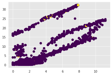
Transactions can be now visualized on a plane (e.g. with different colors for frauds and genuine)
plt.scatter(x_train_representation[:, 0], x_train_representation[:, 1], c=y_train.numpy(), s=50, cmap='viridis')
<matplotlib.collections.PathCollection at 0x7f9f243358e0>
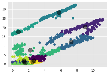
It is also possible to apply a K-means clustering and vizualize the clusters:
from sklearn.cluster import KMeans

kmeans = KMeans(n_clusters=10, random_state=SEED)
kmeans.fit(x_train_representation)
y_kmeans = kmeans.predict(x_train_representation)
plt.scatter(x_train_representation[:, 0], x_train_representation[:, 1], c=y_kmeans, s=50, cmap='viridis')

centers = kmeans.cluster_centers_
plt.scatter(centers[:, 0], centers[:, 1], c='black', s=200, alpha=0.5)
<matplotlib.collections.PathCollection at 0x7f9f25e1c460>
3.7. Semi-supervised fraud detection
Finally, the autoencoder can be used in a semi-supervised credit card fraud detection system [CLBC+19]. There are two main ways to do this:
W1: The most natural one is to keep the autoencoder as is and train it on all available labeled and unlabeled data. Then, to combine it with a supervised neural network trained only on labeled data. The combination can be done by aggregating the predicted score from the supervised model and the predicted score from the unsupervised model (W1A), or more elegantly by providing the unsupervised risk score from the autoencoder (reconstruction error) as an additional variable to the supervised model (W1B) as in [AHJ+20].W2: Another possibility is to change the architecture of the autoencoder into a hybrid semi-supervised model. More precisely, one can add, to the autoencoder, output neurons similar to those of the supervised neural network from the previous section, and additionally predict them from the code neurons. Therefore, the learned representation (code neurons) will be shared between the decoder network that aims at reconstructing the input and the prediction network that aims at predicting fraud. The first is trained on all samples and the latter is only trained on labeled samples. The intuition with this approach is similar to pre-training in natural language processing: learning a representation that embeds the underlying structure in the input data can help with solving supervised tasks.
The following explores the W1B semi-supervised approach. But first, let us reevaluate here the baseline supervised model without the reconstruction error feature. FraudDataset and SimpleFraudMLPWithDropout are available in the shared functions and can be directly used here.
seed_everything(SEED)

training_set_supervised = FraudDataset(x_train.to(DEVICE), y_train.to(DEVICE))
valid_set_supervised = FraudDataset(x_valid.to(DEVICE), y_valid.to(DEVICE))

training_generator_supervised,valid_generator_supervised = prepare_generators(training_set_supervised,
                                                                              valid_set_supervised,
                                                                              batch_size=64)

model_supervised = SimpleFraudMLPWithDropout(len(input_features), 1000, 0.2).to(DEVICE)
optimizer = torch.optim.Adam(model_supervised.parameters(), lr = 0.0001)
criterion = torch.nn.BCELoss().to(DEVICE)

model_supervised,training_execution_time,train_losses_dropout,valid_losses_dropout =\
    training_loop(model_supervised,
                  training_generator_supervised,
                  valid_generator_supervised,
                  optimizer,
                  criterion,
                  verbose=True)
Epoch 0: train loss: 0.10161001316804161
valid loss: 0.03556653917487202
New best score: 0.03556653917487202

Epoch 1: train loss: 0.03833597035852419
valid loss: 0.026109349807022047
New best score: 0.026109349807022047

Epoch 2: train loss: 0.031094471842315882
valid loss: 0.02396169698420566
New best score: 0.02396169698420566

Epoch 3: train loss: 0.028757975434966342
valid loss: 0.023352081602938026
New best score: 0.023352081602938026

Epoch 4: train loss: 0.02775647486163834
valid loss: 0.022305768956761052
New best score: 0.022305768956761052

Epoch 5: train loss: 0.026740792337858456
valid loss: 0.021572637600223713
New best score: 0.021572637600223713

Epoch 6: train loss: 0.02606928332959859
valid loss: 0.021479292579320935
New best score: 0.021479292579320935

Epoch 7: train loss: 0.025758702903594215
valid loss: 0.02105785213192019
New best score: 0.02105785213192019

Epoch 8: train loss: 0.02527676529854707
valid loss: 0.020694473186187202
New best score: 0.020694473186187202

Epoch 9: train loss: 0.024878843686695656
valid loss: 0.02042211337890374
New best score: 0.02042211337890374

Epoch 10: train loss: 0.02438850605296751
valid loss: 0.020538174796116644
1  iterations since best score.

Epoch 11: train loss: 0.024034218137004692
valid loss: 0.02071835831255535
2  iterations since best score.

Epoch 12: train loss: 0.023670860127248512
valid loss: 0.01998928964819983
New best score: 0.01998928964819983

Epoch 13: train loss: 0.023701557650517523
valid loss: 0.01986558492743293
New best score: 0.01986558492743293

Epoch 14: train loss: 0.02331948666341414
valid loss: 0.01986974315244521
1  iterations since best score.

Epoch 15: train loss: 0.023050426844735388
valid loss: 0.01970138840245012
New best score: 0.01970138840245012

Epoch 16: train loss: 0.022976456373844503
valid loss: 0.01949228905777503
New best score: 0.01949228905777503

Epoch 17: train loss: 0.022786046317435738
valid loss: 0.01982322550668824
1  iterations since best score.

Epoch 18: train loss: 0.022582473735731044
valid loss: 0.01974369095577324
2  iterations since best score.

Epoch 19: train loss: 0.02253310805256523
valid loss: 0.019359889266824176
New best score: 0.019359889266824176

Epoch 20: train loss: 0.022279470434334897
valid loss: 0.01928481163261102
New best score: 0.01928481163261102

Epoch 21: train loss: 0.02220114628115694
valid loss: 0.018997078554964335
New best score: 0.018997078554964335

Epoch 22: train loss: 0.022127013866091592
valid loss: 0.01905235069170289
1  iterations since best score.

Epoch 23: train loss: 0.022129482317989224
valid loss: 0.018972578141940095
New best score: 0.018972578141940095

Epoch 24: train loss: 0.02179307807468405
valid loss: 0.01934589187568817
1  iterations since best score.

Epoch 25: train loss: 0.021895541540831398
valid loss: 0.018781205812657426
New best score: 0.018781205812657426

Epoch 26: train loss: 0.02153568957303695
valid loss: 0.018873276155635388
1  iterations since best score.

Epoch 27: train loss: 0.021719574671969652
valid loss: 0.01871486084059878
New best score: 0.01871486084059878

Epoch 28: train loss: 0.021623164488258195
valid loss: 0.01849896589324611
New best score: 0.01849896589324611

Epoch 29: train loss: 0.021195488194819277
valid loss: 0.018997153041558596
1  iterations since best score.

Epoch 30: train loss: 0.021170051902644763
valid loss: 0.01968524302457729
2  iterations since best score.

Epoch 31: train loss: 0.02115491109416708
valid loss: 0.01879670942823092
3  iterations since best score.
Early stopping
predictions = []

for x_batch, y_batch in valid_generator_supervised:
    predictions.append(model_supervised(x_batch.to(DEVICE)).detach().cpu().numpy())

predictions_df=valid_df
predictions_df['predictions']=np.vstack(predictions)

performance_assessment(predictions_df, top_k_list=[100])
| AUC ROC | Average precision | Card Precision@100 | |
|---|---|---|---|
| 0 | 0.859 | 0.646 | 0.28 |
Now, for the W1B semi-supervised approach, let us compute the reconstruction error of all transactions with our first autoencoder (stored in model) and add it as a new variable in train_df and valid_df.
loader_params = {'batch_size': 64,
                 'num_workers': 0}

training_generator = torch.utils.data.DataLoader(training_set, **loader_params)
valid_generator = torch.utils.data.DataLoader(valid_set, **loader_params)

train_reconstruction = per_sample_mse(model, training_generator)
valid_reconstruction = per_sample_mse(model, valid_generator)

train_df["reconstruction_error"] = train_reconstruction
valid_df["reconstruction_error"] = valid_reconstruction
Then, we can reevaluate the supervised model with this extra variable.
seed_everything(SEED)

input_features_new = input_features + ["reconstruction_error"]

# Rescale the reconstruction error
(train_df, valid_df)=scaleData(train_df, valid_df, ["reconstruction_error"])

x_train_new = torch.FloatTensor(train_df[input_features_new].values)
x_valid_new = torch.FloatTensor(valid_df[input_features_new].values)

training_set_supervised_new = FraudDataset(x_train_new.to(DEVICE), y_train.to(DEVICE))
valid_set_supervised_new = FraudDataset(x_valid_new.to(DEVICE), y_valid.to(DEVICE))

training_generator_supervised,valid_generator_supervised = prepare_generators(training_set_supervised_new,
                                                                              valid_set_supervised_new,
                                                                              batch_size=64)

model_supervised = SimpleFraudMLPWithDropout(len(input_features_new), 100, 0.2).to(DEVICE)
optimizer = torch.optim.Adam(model_supervised.parameters(), lr = 0.0001)
criterion = torch.nn.BCELoss().to(DEVICE)

model_supervised,training_execution_time,train_losses_dropout,valid_losses_dropout = \
    training_loop(model_supervised,
                  training_generator_supervised,
                  valid_generator_supervised,
                  optimizer,
                  criterion,
                  verbose=True)

predictions = []
for x_batch, y_batch in valid_generator_supervised:
    predictions.append(model_supervised(x_batch).detach().cpu().numpy())
Epoch 0: train loss: 0.32470558333009425
valid loss: 0.11669875736770734
New best score: 0.11669875736770734

Epoch 1: train loss: 0.0857971908175609
valid loss: 0.050325598816076914
New best score: 0.050325598816076914

Epoch 2: train loss: 0.055031552282206526
valid loss: 0.03683824896140665
New best score: 0.03683824896140665

Epoch 3: train loss: 0.045474566717366785
valid loss: 0.031574366707863705
New best score: 0.031574366707863705

Epoch 4: train loss: 0.03988730701053405
valid loss: 0.028506962655753386
New best score: 0.028506962655753386

Epoch 5: train loss: 0.03588366161686427
valid loss: 0.0264507318495727
New best score: 0.0264507318495727

Epoch 6: train loss: 0.03320539464736019
valid loss: 0.025167095382784395
New best score: 0.025167095382784395

Epoch 7: train loss: 0.03146339780281531
valid loss: 0.024275742485722313
New best score: 0.024275742485722313

Epoch 8: train loss: 0.03083236553407066
valid loss: 0.02372574291110568
New best score: 0.02372574291110568

Epoch 9: train loss: 0.029903344949351242
valid loss: 0.023402261280561568
New best score: 0.023402261280561568

Epoch 10: train loss: 0.029085144788573495
valid loss: 0.02301961904330576
New best score: 0.02301961904330576

Epoch 11: train loss: 0.02864163257867226
valid loss: 0.022839933189008732
New best score: 0.022839933189008732

Epoch 12: train loss: 0.028412688680235332
valid loss: 0.022551339802133745
New best score: 0.022551339802133745

Epoch 13: train loss: 0.02834755417122461
valid loss: 0.022378979152821697
New best score: 0.022378979152821697

Epoch 14: train loss: 0.028343526197305343
valid loss: 0.022222696035805213
New best score: 0.022222696035805213

Epoch 15: train loss: 0.027864306476447966
valid loss: 0.022193545799402144
New best score: 0.022193545799402144

Epoch 16: train loss: 0.027414113502855098
valid loss: 0.0219534132029108
New best score: 0.0219534132029108

Epoch 17: train loss: 0.027424028700433072
valid loss: 0.02181996635156251
New best score: 0.02181996635156251

Epoch 18: train loss: 0.02662210316247223
valid loss: 0.021762580478747115
New best score: 0.021762580478747115

Epoch 19: train loss: 0.026635378260048814
valid loss: 0.02163417828167519
New best score: 0.02163417828167519

Epoch 20: train loss: 0.026724288395666526
valid loss: 0.02153022467486988
New best score: 0.02153022467486988

Epoch 21: train loss: 0.0266051148182408
valid loss: 0.021428093735047213
New best score: 0.021428093735047213

Epoch 22: train loss: 0.02637773595953335
valid loss: 0.021339995185513803
New best score: 0.021339995185513803

Epoch 23: train loss: 0.026257544278254445
valid loss: 0.021252412970885228
New best score: 0.021252412970885228

Epoch 24: train loss: 0.026126052476430087
valid loss: 0.021180965348218103
New best score: 0.021180965348218103

Epoch 25: train loss: 0.02579458606234408
valid loss: 0.021089692087589554
New best score: 0.021089692087589554

Epoch 26: train loss: 0.025870972849209625
valid loss: 0.02096897741255498
New best score: 0.02096897741255498

Epoch 27: train loss: 0.02589873712250329
valid loss: 0.02103838359115167
1  iterations since best score.

Epoch 28: train loss: 0.025474642118506745
valid loss: 0.02083245238971189
New best score: 0.02083245238971189

Epoch 29: train loss: 0.025491673881757868
valid loss: 0.020914757669053444
1  iterations since best score.

Epoch 30: train loss: 0.0256901814166704
valid loss: 0.02079701650928441
New best score: 0.02079701650928441

Epoch 31: train loss: 0.025314893825050894
valid loss: 0.02063066685404323
New best score: 0.02063066685404323

Epoch 32: train loss: 0.025559447194898346
valid loss: 0.02062068326803321
New best score: 0.02062068326803321

Epoch 33: train loss: 0.024862300820050344
valid loss: 0.020600306137866987
New best score: 0.020600306137866987

Epoch 34: train loss: 0.025080274871548718
valid loss: 0.020477301164280846
New best score: 0.020477301164280846

Epoch 35: train loss: 0.024728723903396744
valid loss: 0.020394465477394114
New best score: 0.020394465477394114

Epoch 36: train loss: 0.02477897367222915
valid loss: 0.020449772248645134
1  iterations since best score.

Epoch 37: train loss: 0.024465490879030653
valid loss: 0.020325674156434426
New best score: 0.020325674156434426

Epoch 38: train loss: 0.024305174552148163
valid loss: 0.020269202150511326
New best score: 0.020269202150511326

Epoch 39: train loss: 0.024521953303208416
valid loss: 0.020168634172646034
New best score: 0.020168634172646034

Epoch 40: train loss: 0.024144744264793513
valid loss: 0.020071419583928714
New best score: 0.020071419583928714

Epoch 41: train loss: 0.024092775663578203
valid loss: 0.020062985963854797
New best score: 0.020062985963854797

Epoch 42: train loss: 0.02412362778172018
valid loss: 0.020077789380454302
1  iterations since best score.

Epoch 43: train loss: 0.023811501132976087
valid loss: 0.01995381725687391
New best score: 0.01995381725687391

Epoch 44: train loss: 0.02424977031820427
valid loss: 0.019959632811630195
1  iterations since best score.

Epoch 45: train loss: 0.02389407654877852
valid loss: 0.0198583653335373
New best score: 0.0198583653335373

Epoch 46: train loss: 0.023958714262081085
valid loss: 0.01977933693201347
New best score: 0.01977933693201347

Epoch 47: train loss: 0.023485491898673876
valid loss: 0.019806338451762016
1  iterations since best score.

Epoch 48: train loss: 0.023657646779875568
valid loss: 0.019662209351603045
New best score: 0.019662209351603045

Epoch 49: train loss: 0.023470603387796607
valid loss: 0.01968898415804683
1  iterations since best score.

Epoch 50: train loss: 0.02365986756685708
valid loss: 0.019617491648048976
New best score: 0.019617491648048976

Epoch 51: train loss: 0.02301738877784297
valid loss: 0.01950973152880216
New best score: 0.01950973152880216

Epoch 52: train loss: 0.023529816942643837
valid loss: 0.019513023327883395
1  iterations since best score.

Epoch 53: train loss: 0.023395457049479162
valid loss: 0.01949332637045675
New best score: 0.01949332637045675

Epoch 54: train loss: 0.02303883458951125
valid loss: 0.01939637301988452
New best score: 0.01939637301988452

Epoch 55: train loss: 0.022967305407017097
valid loss: 0.01937846771538095
New best score: 0.01937846771538095

Epoch 56: train loss: 0.023021493925660472
valid loss: 0.01932469207037729
New best score: 0.01932469207037729

Epoch 57: train loss: 0.02324649085298298
valid loss: 0.019319333965365924
New best score: 0.019319333965365924

Epoch 58: train loss: 0.02314090387805331
valid loss: 0.01927059471538504
New best score: 0.01927059471538504

Epoch 59: train loss: 0.022600235849646513
valid loss: 0.019282025675024694
1  iterations since best score.

Epoch 60: train loss: 0.022965760435352554
valid loss: 0.019262573485965002
New best score: 0.019262573485965002

Epoch 61: train loss: 0.023083728506856634
valid loss: 0.019118402978720885
New best score: 0.019118402978720885

Epoch 62: train loss: 0.022604351701886245
valid loss: 0.019093919451643657
New best score: 0.019093919451643657

Epoch 63: train loss: 0.02272556185217959
valid loss: 0.01905925034906695
New best score: 0.01905925034906695

Epoch 64: train loss: 0.0222361646619328
valid loss: 0.01899794363760252
New best score: 0.01899794363760252

Epoch 65: train loss: 0.022313779764221074
valid loss: 0.018973210823080944
New best score: 0.018973210823080944

Epoch 66: train loss: 0.022522902168711046
valid loss: 0.018901191251937687
New best score: 0.018901191251937687

Epoch 67: train loss: 0.02248352280253434
valid loss: 0.01889178021709165
New best score: 0.01889178021709165

Epoch 68: train loss: 0.022433675548692106
valid loss: 0.018912809526501987
1  iterations since best score.

Epoch 69: train loss: 0.02257502525739895
valid loss: 0.018815524044034422
New best score: 0.018815524044034422

Epoch 70: train loss: 0.0224518446423368
valid loss: 0.018792384044302862
New best score: 0.018792384044302862

Epoch 71: train loss: 0.02226468713430556
valid loss: 0.018732086603804567
New best score: 0.018732086603804567

Epoch 72: train loss: 0.022387760058183395
valid loss: 0.01883075698622365
1  iterations since best score.

Epoch 73: train loss: 0.022133301173819384
valid loss: 0.01867632728383006
New best score: 0.01867632728383006

Epoch 74: train loss: 0.022178997785715745
valid loss: 0.018700476872729636
1  iterations since best score.

Epoch 75: train loss: 0.022028937389144593
valid loss: 0.018650301263280863
New best score: 0.018650301263280863

Epoch 76: train loss: 0.02214035027425373
valid loss: 0.018606594060496758
New best score: 0.018606594060496758

Epoch 77: train loss: 0.021738268898102858
valid loss: 0.018632269502983842
1  iterations since best score.

Epoch 78: train loss: 0.02227861989753848
valid loss: 0.01854319557435607
New best score: 0.01854319557435607

Epoch 79: train loss: 0.021809139837872374
valid loss: 0.018610031961443035
1  iterations since best score.

Epoch 80: train loss: 0.022240891229284725
valid loss: 0.018547307454874037
2  iterations since best score.

Epoch 81: train loss: 0.022066849491217958
valid loss: 0.01848699482949196
New best score: 0.01848699482949196

Epoch 82: train loss: 0.021692594942564668
valid loss: 0.018455498772571525
New best score: 0.018455498772571525

Epoch 83: train loss: 0.02205857191164488
valid loss: 0.01839941353727987
New best score: 0.01839941353727987

Epoch 84: train loss: 0.021860865075639797
valid loss: 0.0183856724618929
New best score: 0.0183856724618929

Epoch 85: train loss: 0.021753365356460868
valid loss: 0.018383686461923593
New best score: 0.018383686461923593

Epoch 86: train loss: 0.021993174024765874
valid loss: 0.018376381002758412
New best score: 0.018376381002758412

Epoch 87: train loss: 0.021596283111213768
valid loss: 0.018388316551951153
1  iterations since best score.

Epoch 88: train loss: 0.021463176303113105
valid loss: 0.018383121337420993
2  iterations since best score.

Epoch 89: train loss: 0.02156794395123699
valid loss: 0.0182802003695085
New best score: 0.0182802003695085

Epoch 90: train loss: 0.021446433153811905
valid loss: 0.018424906315602608
1  iterations since best score.

Epoch 91: train loss: 0.02153544440147882
valid loss: 0.01828304048184855
2  iterations since best score.

Epoch 92: train loss: 0.02158625805340921
valid loss: 0.01830057208871601
3  iterations since best score.
Early stopping
predictions_df=valid_df
predictions_df['predictions']=np.vstack(predictions)

performance_assessment(predictions_df, top_k_list=[100])
| AUC ROC | Average precision | Card Precision@100 | |
|---|---|---|---|
| 0 | 0.861 | 0.651 | 0.276 |
The three metrics are very close, with or without the additional feature. They respectively went from 0.859, 0.646 and 0.28 to 0.861, 0.651 and 0.276. The conclusion is therefore mitigated and does not show a significant benefit from this semi-supervised modeling. Nevertheless, keep in mind that, in practice in a different setting, there can be a benefit, especially if the quantity of available unlabeled data is much larger than the quantity of labeled data.
Also, note that there are several directions for improvement. For example, this semi-supervised technique can be pushed further by training two separate autoencoders, for each class, and by using both reconstruction errors as additional variables.
3.8. Conclusion
Autoencoders are part of the large deep learning models family. Their goal is to learn representations to reconstruct descriptive variables, so they have been widely used for unsupervised learning problems. Anomaly detection, and in particular fraud detection, can be tackled with unsupervised or semi-supervised techniques.
In this section, we used the autoencoder, and in particular its reconstruction error, as an indicator for fraud risk. Used solely (unsupervised method), it detects data points that are away from the rest of the distribution, which allows detecting many frauds but also introduces a lot of false alerts (e.g. genuine transactions that have rare characteristics). Therefore, it obtains a decent AUC ROC but low precision-based metrics. Used as an extra variable in a supervised method (semi-supervised usage), it can allow boosting the performance in specific settings.